Technical documentation

Context

Overview of the model

The Res-IRF model1 is a tool for simulating energy consumption and energy efficiency improvements in the French residential building sector. It currently focuses on space heating as the main usage. The rationale for its development is to integrate a detailed description of the energy performance of the dwelling stock with a rich description of household behaviour. Res-IRF has been developed to improve the behavioural realism that is typically lacking in integrated models of energy demand.

Fed by population growth, household income growth and energy prices as exogenous inputs, the model returns construction and renovation costs and flows, energy consumption and heating comfort as endogenous outputs (Fig. 7). This process is iterated on an annual time-step basis. The energy efficiency of a dwelling is characterized by its Energy Performance Certificate (EPC, diagnostic de performance énergétique ) and energy efficiency improvements correspond to upgrade to one a more efficient label. Energy consumption results from household decisions along three margins: the extensive margin of investment – the decision of whether or not to renovate –, the intensive margin of investment – the magnitude of the energy efficiency upgrade – and the intensity with which the heating infrastructure is used after renovation. Investment decisions are based on a net present value (NPV) calculation that incorporates a number of barriers at the source of the so-called ‘energy-efficiency gap’ – the discrepancy between observed energy-efficiency levels and those predicted by engineering studies[Jaffe and Stavins, 1994], [Gillingham, Newell, and Palmer, 2009], [Allcott and Greenstone, 2012]. These include: myopic expectation of energy prices, hidden costs of renovation (e.g., inconvenience associated with insulation works), barriers to collective decision-making within homeowner associations, split incentives between landlords and tenants, credit constraints, and the so-called rebound effect.

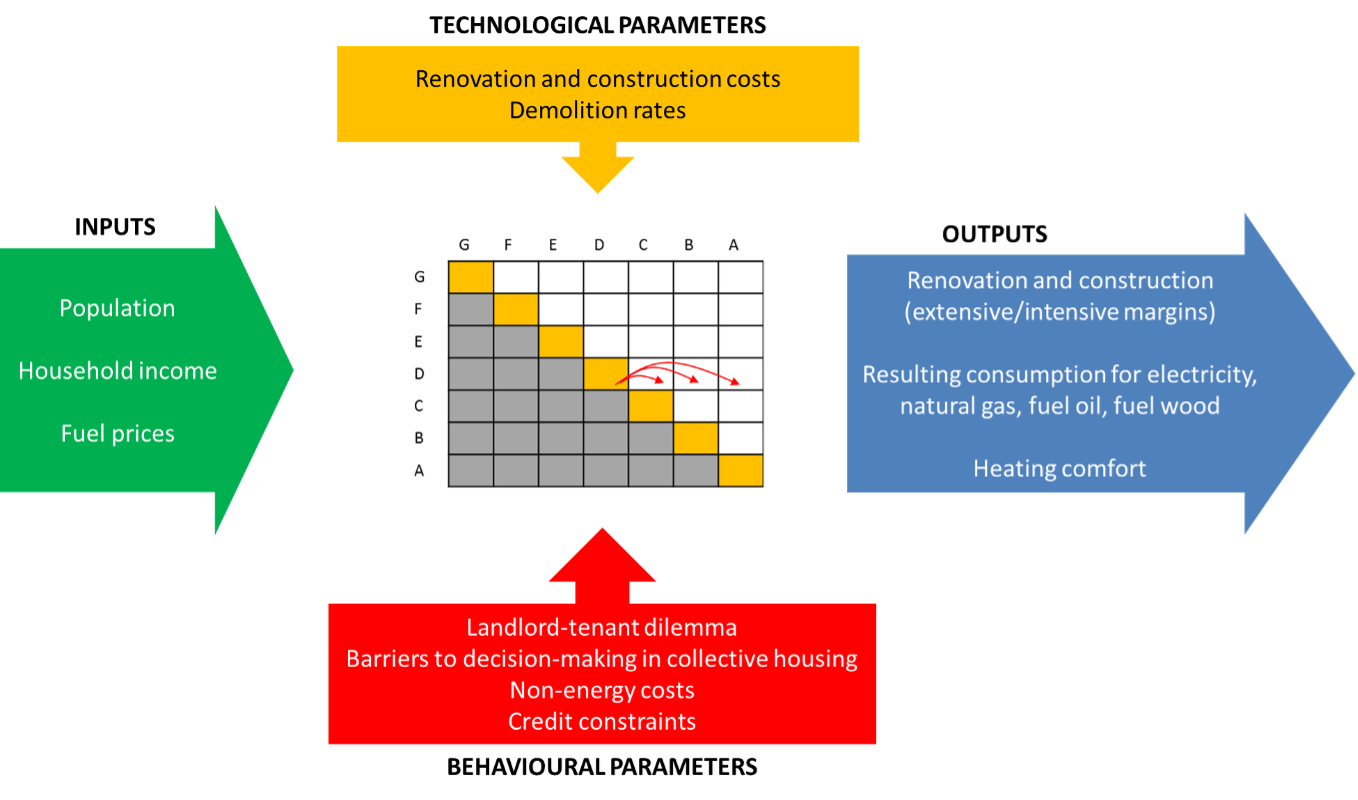
Fig. 7 Elementary structure model

Previous developments

The development of Res-IRF has produced six peer-reviewed articles to this day, of which an overview is provided in Table 23.

Overview of achievements with Res-IRF

Table 23 Previous Developments
Version	Peer-reviewed publications	Approach	Main results	Main data source	Main additions to preceding version
1	Giraudet et al., Energy Journal, 2011	Policy analysis	Policy portfolio considered (energy efficiency subsidies, carbon tax, building codes) does not permit attainment of sectoral energy saving targets	ANAH (2008)
	Giraudet et al., Energy Economics, 2012*	Sensitivity analysis	Business as usual reduction in energy use of 37% to 2050, with an additional 21% if barriers to energy efficiency are removed
	Mathy et al., Energy Policy, 2015	Policy analysis	Carbon dioxide emission reductions of 58% to 81% by 2050
2	Branger et al., Environmental Modelling & Software, 2015*	Sensitivity analysis	Monte Carlo simulations point to 13% overall uncertainty in model outputs. Morris method of elementary effects identifies energy prices as the most influential variable.		Updating of retrofit costs and heating intensity parameters; introduction of fuel wood and social housing.
3	Giraudet et al., working paper, 2018	Policy analysis	Policy interactions imply a 10% variation in policy effectiveness	Phébus (2013)	Comprehensive updating of model parameters; calibration on base year 2012 ; disaggregation of households by income categories.
	Bourgeois et al., ECEEE proceedings, 2019	Policy analysis	Carbon tax generates more environmental, social and economic benefits when its revenue is recycled as energy efficiency subsidies than as a lump-sum transfer
3.1	Glotin et al., Energy Economics, 2019*	Backtesting	Model reproduces past energy consumption with an average percentage error of 1.5%. Analysis reveals inaccuracies in fuel switch due to off-model, politically-driven processes	CEREN archives	Calibration of version 3.0 on base year 1984 (instead of 2012).
3	Giraudet et al., Energy Policy, 2021*	Policy analysis	Carbon tax is the most effective, yet most regressive, policy. Subsidy programmes save energy at a cost of €0.05–0.08	Phébus (2013)
3	Bourgeois et al., Ecological Economics, 2021	Policy analysis	Subsidy recycling saves energy and increases comfort more cost-effectively than lump-sum	Phébus (2013)

Note : The symbol * points to the reference that contains the most comprehensive description of the associated version of the model. The most comprehensive description of version 3.0 is to be found in the present document.

The documentation reflects the latest version of the model. The model is intended to be input-agnostic and the documentation is structured to reflect this paradigm. For the sake of clarity, however, some processes are illustrated with numerical examples from version 3.0, which was used in several recent publications.

Scilab to Python

The model was initally coded in Scilab language. It was recently re-coded in the more popular Python language to gain more visibility. This recoding procedure implied changes in the model structure, due for instance to errors that had not been detected in the previous version. To assess the importance of these changes, we ran the Scilab and Python version of Res-IRF 3.0 and examined the differences among them across a range of outputs. Fig. 8 and Fig. 9 illustrate these differences for two key outputs. We find that, over the range of outputs considered, the difference never exceeds 1% at the 2030 horizon and 5% at the 2050 horizon. We conclude that the errors are negligible and therefore validate the Python version of Res-IRF 3.0.

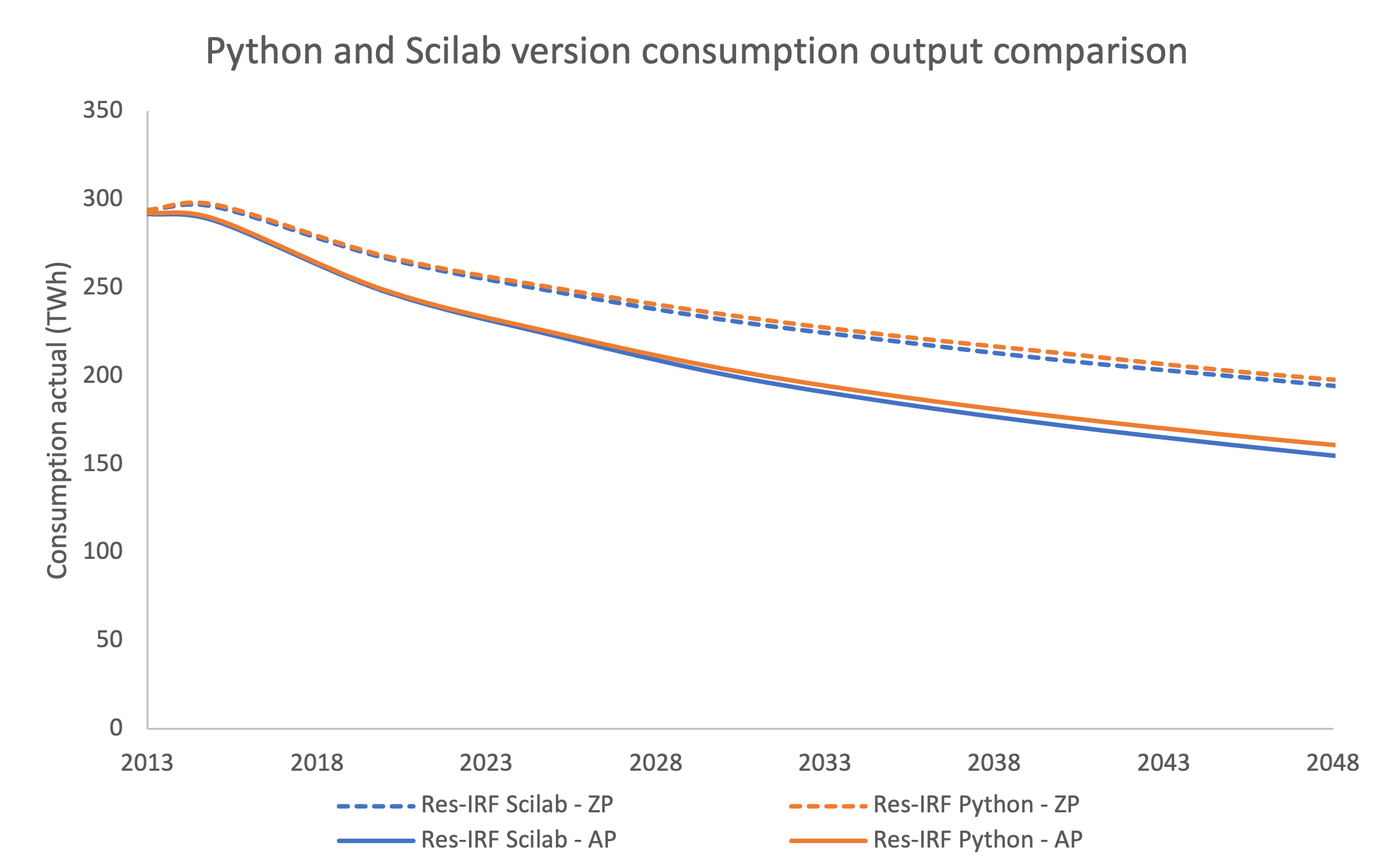
_images/res_irf_python_comparison_comsumption.png

Fig. 8 Python/Scilab consumption output comparison.

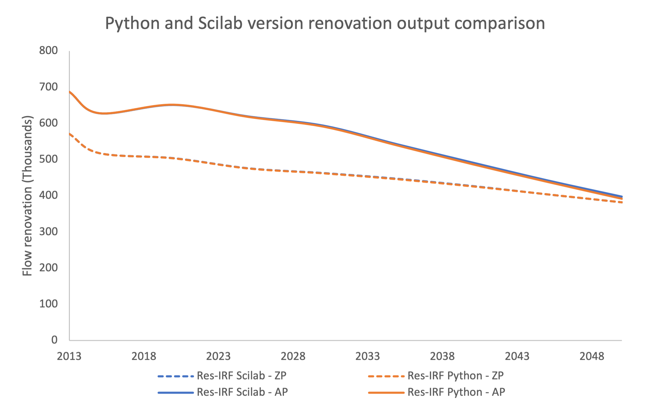
_images/res_irf_python_comparison_renovation.png

Fig. 9 Python/Scilab renovation output comparison.

Table 24 Comparison Scilab/Python
Zero politics			2013	2015	2020	2025	2030	2035	2040	2045	2050
Consumption actual (TWh)	Res-IRF Scilab - ZP	TWh	294	296	267	248	232	220	209	200	191
Consumption actual (TWh)	Res-IRF Python - ZP	TWh	294	297	268	250	235	223	213	203	195
			0.00%	0.34%	0.37%	0.81%	1.29%	1.36%	1.91%	1.50%	2.09%

Flow renovation (Thousands)	Res-IRF Scilab - ZP	milliers	571	518	504	476	463	447	427	404	382
Flow renovation (Thousands)	Res-IRF Python - ZP	milliers	571	518	504	476	463	446	426	404	382
			0.07%	0.07%	-0.01%	-0.03%	-0.08%	-0.17%	-0.12%	0.12%	0.10%
All politics
Consumption actual (TWh)	Res-IRF Scilab - AP	TWh	292	288	248	223	201	185	172	161	151
Consumption actual (TWh)	Res-IRF Python - AP	TWh	292	289	249	225	204	189	177	167	158
			0.15%	0.33%	0.30%	0.71%	1.62%	2.20%	2.85%	3.49%	4.46%

Flow renovation (Thousands)	Res-IRF Scilab - AP	milliers	687	628	651	619	594	542	492	443	398
Flow renovation (Thousands)	Res-IRF Python - AP	milliers	687	628	652	618	591	539	487	439	392
			0.00%	0.02%	0.09%	-0.20%	-0.47%	-0.61%	-0.97%	-0.99%	-1.52%

Energy use

The model uses two metrics for energy use: the conventional consumption predicted by the EPC label of the dwelling; and the actual consumption that determines energy expenditure. The two are linked by the intensity of heating of the heating infrastructure, which is an endogenous function of the model.

Conventional energy use

Integrating new data on specific consumption (kWh/m²/year) and housing surface area (m²) allowed us to improve the accuracy of total consumption parameters (kWh/year).

Specific consumption

The conventional specfic consumption of an existing dwelling is directly given by its EPC label2. By including a precise measurement of the conventional energy consumption of each dwelling, the Phébus-DPE database made it possible to estimate for each band an average consumption.

Since the EPC covers energy consumption for heating, hot water and air conditioning, adjustments are needed to isolate the part specifically dedicated to heating. Here again, the Phébus-DPE database, by distinguishing energy between heating use, hot water use and photovoltaic production, makes it possible to estimate an average share dedicated to heating for each EPC band.

Table 25 Conventional primary energy consumption
EPC band	Average consumption (kWh/m²/year)	Share dedicated to heating	Average consumption for heating in Res-IRF (kWh/m²/an)
G	596	0.85	507
F	392	0.82	321
E	280	0.77	216
D	191	0.74	141
C	125	0.72	90
B	76	0.77	59
A	40	1.12	45
LE	50	0.4	20
NZ	40	0.4	16

New dwellings fall into two categories of energy performance:

Low Energy (LE) level, aligned with the prevailing building code at 50 kWh/m²/year of primary energy,
Net Zero Energy (NZ) level, mandating zero consumption, net of production from renewable sources. Since we focus on gross energy consumption, we assign a consumption of 40 kWhEP/m²/year to NZ dwellings.

The same coefficient of 0.4 is applied to BBC and BEPOS consumption in order to isolate heating from the five usages covered by building code prescriptions (instead of three usages in the case of the EPC in existing dwellings). Note that the energy requirements of EPC band A are also net of production from renewable sources. Our focus on gross consumption leads us to apply a coefficient that is greater than 1. These calculations are detailed in Table 25.

Surface area

The same approach was used to set surface area parameters bases on average values estimated on Phébus data, by category of dwelling.

Actual energy use

A growing number of academic studies point to a gap between the conventional energy consumption predicted by energy performance certificates and actual energy consumption. The most common explanation is a more intense heating of the heating infrastructure after an energy efficiency improvement – a phenomenon commonly referred to as the “rebound effect.” 3

In version 3.0, we included a third variable: household income. This development was made possible by several improvements in the data available, including the Phébus database and additional work by EDF R&D [Cayla and Osso, 2013], which now connects heating intensity to the income share devoted to heating, i.e. conventional expenditure as a percentage of income.

Heating intensity in Res-IRF follows the equation:

\[\text{Heating Intensity} =-0,191*log(\text{Income share})+0,1105\]

with:

\[\text{Heating Intensity} = \frac{\text{Actual energy use}}{\text{Conventional energy use}}\]

and:

\[\text{Income share} =\frac{\text{Energy price} * \text{Surface}* \text{Conventional energy use}}{\text{Income}}\]

Total energy use

The total final actual energy consumption generated by Res-IRF from data for the initial year differs from the values produced by CEREN. These differences are due to differing scopes between the initial building stock and CEREN databases and to the adjustments needed to select the main heating fuel.

To ensure consistency with the CEREN data, which is the reference commonly used in modelling exercises, Res-IRF is calibrated to reproduce the final energy consumption given by CEREN for each fuel in the initial year. The resulting conversion coefficients applied to the Phebus Building Stock are listed in Table 26. They indicate that Res-IRF reproduces natural gas and heating oil consumption fairly accurately, with an error of around 5%. On the other hand, electricity consumption is clearly overestimated and fuel-wood consumption is greatly underestimated. The succinct documentation of the CEREN database did not allow us to clearly identify the reasons for these biases. However, it can reasonably be assumed that they are attributable to the procedure for selecting a main heating fuel in Res-IRF, which probably implies some substitution of electricity for wood in dwellings that are mainly heated with electricity but use wood as auxiliary heating. The difficulties inherent in converting different forms of wood (logs, pellets, etc.) into TWh can also explain the differences observed in wood consumption.

Table 26 Calibration of total final actual energy consumption
	Electricity	Natural gas	Fuel oil	Fuel wood	TOTAL
CEREN values to be reproduced in 2012 (TWhEF)	44.4	119.7	55.5	73.3	292.9
Correction factor applied to Res-IRF 3.0	0.79	1.06	1.03	2.14	1.14

Energy efficiency improvements

Stock dynamics

The number of dwellings and their surface area are determined each year in Res-IRF by exogenous projections of population and aggregate household income projection. The former is based on [INSEE, 2006]; in the absence of an authoritative scenario, the latter is based on a growth assumption of 1.2%/year, which extrapolates the trend given by INSEE for the period 2009-20134. Based on the annual needs thus determined, the total housing stock is divided into two components:

The stock of “existing dwellings” corresponds to the total stock of the initial year. It is eroded at a rate of 0.35%/year due to destruction, based on [Allaire, Gaudière, Majchrzak, and Masi, 2008]. Destructions are assumed to affect in priority the lowest energy performance labels, based on based on [Traisnel, 2001].
New constructions are calculated to match housing needs, determined by total projected housing needs net of the existing stock. The cumulative sum of new constructions since the initial year constitutes the stock of “new dwellings.”

This specification produces a flow of new constructions of 365,000 in 2013, 357,000 in 2014 and 348,000 in 2015, similar to the average of 374,000 given by [INSEE, 2018] over a slightly wider area including the French overseas departments and territories, except Mayotte.

Res-IRF reflects thanks to recent empirical work linking the increase in the share of multi-family housing in the total stock to the rate of growth of the total stock housing growth [Fisch, Marfaing, and Rognant, 2015]. This relationship in particular reflects urbanization effects. The share of owner-occupied and rented dwellings is held constant.

Investment decisions – general case

The energy performance of the housing stock in Res-IRF is affected by both the construction of new dwellings and the renovation of existing ones. Both effects are modelled by discrete choice functions. Generally speaking, the owner of a dwelling of initial performance i∈{1…n} chooses to upgrade it to an option of final performance f∈{i+1,…,n} by comparing its life-cycle cost to that of other options. The life-cycle cost \(LCC_{i,f}\) of an option is the sum of three terms:

\[LCC_{i,f}= INV_{i,f}+ γ * ENER_f + IC_{i,f}\]

where INV is the investment cost; ENER is the life-cycle discounted cost of conventional energy use, calculated using the energy price for the year under consideration; IC are some “intangible costs,” representing non-energy attributes of the investment, such as aesthetic or acoustic benefits, inconvenience generated by insulation works, etc…

The assumption of myopic expectation, which materializes by applying the discount factor to the contemporaneous energy price, is justified by a number of econometric studies [Anderson, Kellogg, and Sallee, 2011] The discount factor γ depends on the discount rate r and the investment horizon l according to the following relationship:

\[γ(r,l)=∑_{t=0} (1+r)^{-t} = \frac{1-(1+r)^{-l)}}{r}\]

The two parameters are set in Res-IRF to capture various barriers to home renovation:

The discount rate captures both the tighter credit constraints facing lower-income households and the barriers to decision-making within homeowner associations.
The investment horizon reflects the intensity with which real estate and rental markets capitalize the “green value” of the housing, i.e., magnitude of the rental or resale premium for a property that has just undergone energy efficiency improvements.

The market share \(MS_{i,f}\) of upgrades from labels i to f, resulting from the aggregation of individual choices, is determined by their life-cycle cost from the following equation:

\[MS_{i,f} = \frac{LCC_{i,f}^{-v}}{∑_{k=i+1} LCC_{i,k} ^{-v}}\]

Parameter v characterizing the heterogeneity of preferences is set to 8 in the model.5 Intangible costs are calibrated so that the observed market shares are reproduced in the initial year.

The paragraphs thereafter describe in detail the specification of energy efficiency improvements, which are based on two types of technical data – the market shares of the different options in the initial year and their investment cost – and two types of behavioural data – the discount rate and the investment horizon.

New constructions

Construction costs at the LE and NZ levels have been updated in Res-IRF 3.0 based on estimates recently made available by CGDD (2015) 6

Table 27 Construction costs (€/m2)
Heating energy final	Power	Power	Natural gas	Natural gas	Oil fuel	Oil fuel	Wood fuel	Wood fuel
Energy performance final	BBC	BEPOS	BBC	BEPOS	BBC	BEPOS	BBC	BEPOS
Single-family	979	1112	1032	1059	1032	1059	1094	1121
Multi-family	1199	1308	1242	1253	1242	1253	1323	1350

The market shares used to calibrate intangible costs were also updated in 3.0, based on trends provided by CEREN.

The massive penetration of natural gas at the expense of electric heating observed over the past ten years in multi-family housing is mainly due to the anticipation and subsequent application of the 2012 building code. In order to abstract from short-term variations, the 2012 market shares are set in Res-IRF on the average of the years 2012-2015 Table 28.

Table 28 Distribution of heating fuels in new constructions in Res-IRF for year 2012
	Electricity	Natural gas	Fuel oil	Fuel wood	Total
Single-family dwellings	75.30%	18.50%	0.50%	5.80%	100%
Multi-family dwellings	19.50%	79.50%	0.00%	1.00%	100%

Considering that the quality of new constructions results from decisions made by building and real estate professionals rather than by future owners, we subject these decisions in the model to private investment criteria, reflected by a discount rate of 7% and a time horizon of 25 years.

Renovation of existing dwellings

The model simultaneously determines the number of renovations and their performance. The process is therefore more complex than in new construction, where the two margins are distinct. For the sake of clarity, we hereafter describe them sequentially.

Intensive margin

Renovation costs \(INV_{i,f}\) are described by an upper diagonal matrix linking the initial EPC label i of the dwelling to its final label f Table 29. Parameterization of the matrix is based on piecemeal data supplemented with values interpolated according to the following principles:

Decreasing returns, i.e., increasing incremental cost of renovation: \(INV_{i,f+2}-INV_{i,f+1} > INV_{i,f+1} - INV_{i,f}\)
Economies of scale, i.e., deep retrofits costing less than a succession of incremental renovations: \(INV_{i,f} < INV_{i,i+k} + INV_{i+k,f}\) for all k such that \(1≤k<f-i\)

Table 29 Renovation costs used in Res-IRF 3.0 (€/m2). Source: Expert opinion
	F	E	D	C	B	A
G	76.0	136.2	200.6	270.7	350.5	441.9
F		63.0	130.3	203.5	286.7	381.8
E			70.0	146.0	232.3	330.9
D				79.0	168.6	270.7
C					93.0	198.9
B						110.0

The matrix equally applies to single- and multi-family dwellings, in both private and social housing.

The same is true for the matrix of market shares used to calibrate intangible costs of renovation, which was based on [PUCA, 2015] (Table 11).

Table 30 Market shares of energy efficiency upgrades in 2012. Source: PUCA (2015)
	F	E	D	C	B	A
G	25.00%	27.00%	27.00%	21.00%	0.00%	0.00%
F		40.40%	26.30%	31.30%	2.00%	0.00%
E			66.00%	28.00%	6.00%	0.00%
D				95.00%	5.00%	0.00%
C					90.90%	9.10%
B						100.00%

Intangible costs are calibrated so that the life-cycle cost model, fed with the investment costs reported in Table 29, matches the market shares reported in Table 30. The resulting intangible costs for Res-IRF 3.0 are reported in Table 31.

Table 31 Averaged intangible costs in 2012 (€/m²)
	F	E	D	C	B	A
G	32	32	51	56	128	149
F		20	43	36	86	125
E			27	33	48	106
D				18	46	74
C					46	36
B						0

The costs reported in Table 29, weighted by the market shares reported in Table 30 and Table 32, result in an average renovation cost of 112 €/m², very close to the 110 €/m² value given by OPEN (9 978 € of average expenditure compared to 91 m²). Compared to the cumulative energy savings they generate (assuming an average lifetime of 26 years), they correspond to an average “negawatt-hour cost” of 83 €/MWh, with extreme values of 25 and 446. These values are in line with those recently produced by [Trésor, 2017].

Extensive margins

An upgrade an initial label i is determined by its net present value (NPV), calculated as the sum of the life-cycle cost of the different options f∈{i+1,…,n}, weighted by their market share:

\[NPV_i=∑_{f>i}^n MS_{i,f} * LCC_{i,f}\]

The renovation rate \(τ_i\) of dwellings labelled i is then calculated as a logistic function of the NPV:

\[τ_i=\frac{τ_{max}}{1+(τ_{max}/τ_{min} -1) e^{-ρ(NPV_i- NPV_{min})}}\]

with \(τ_{min}=0,001%\), \(NPV_{min}=-1 000€\) and \(τ_{max}=20%\). The logistic form captures heterogeneity in heating preference and habits, assuming they are normally distributed7. Parameter ρ is calibrated, for each type of decision-maker and each initial label (i.e., 6x6=36 values), so that the NPVs calculated with the subsidies in effect in 2012 [Giraudet, Guivarch, and Quirion, 2012] reproduce the renovation rates described in Table 32 and Table 33 and their aggregation represents 3% (686,757 units) of the housing stock of the initial year.

Table 33 Renovation rate by type of dwelling. Source : OPEN (2016) and USH (2017)
Type of decision-maker	Type of dwelling	Renovation rate
Owner-occupied	Single-family	4.70%
	Multi-family	3.60%
Privately rented	Single-family	2.00%
	Multi-family	1.80%
Social housing	Single-family	1.50%
	Multi-family	2.00%

Behavioural parameters

Discount rate

In private housing, discount rates are differentiated by housing type in order to capture the heterogeneous constraints faced by investors Table 34. Specifically, the discount rates decrease with the owner’s income to reflect tighter credit constraints faced by lower-income households. Discount rates are also higher in multi-family housing than in single-family homes to capture the difficulties associated with decision-making within homeowner associations. In social housing, on the other hand, the discount rate is set at 4%, the value commonly used in public decision-making.

Table 34 Discount rates. Source: Expert opinion
Income category	Single-family housing	Multi-family housing	Social housing
C1	15%	37%	4%
C2	10%	25%	4%
C3	7%	15%	4%
C4	5%	7%	4%
C5	4%	5%	4%

Investment horizon

The investment horizon is subject to different scenario variants, reflecting different intensities of market capitalization of energy savings Table 35:

In the ‘full capitalization’ scenario, the investment horizon corresponds to the entire lifetime of energy retrofits, i.e., 30 years for improvements on the envelope and 16 years for the improvements on heating systems. Investors enjoy the benefits of the investment as long as they own the property (possibly in the form of higher rents); upon reselling, they receive a premium equal to the discounted sum of the residual monetary savings generated by the investment.
The reference scenario corresponds to a situation where the horizon of landlords is reduced to three years, the average term of a lease. This assumption reflects an inability to increase rents in an attempt to recoup investment. This situation, often referred to as the “landlord-tenant dilemma,” is the most common in practice [Giraudet, Houde, and Maher, 2018].
In the ‘no sale capitalization,’ the investment horizon is limited to seven years, equivalent to the average length of ownership of a property. This assumption totally ignores the residual benefits of the investment at the time of resale.
In the ‘no sale nor rent capitalization’ scenario, the owner-tenant dilemma adds to the lack of capitalization of the resale premium.

Table 35 Investment horizon for improvements on the envelope (on heating systems)
Scenario	Homeowners	Landlords	Social-housing
Full capitalization	30 (16) years	30 (16) years	30 (16) years
Reference	30 (16) years	3 years	30 (16) years
No capitalization at resale	7 years	7 years	30 (16) years
No capitalization in rents nor sales	7 years	3 years	30 (16) years

Endogenous technical change

In both new construction and renovation, the life-cycle costs of the various energy efficiency options decrease endogenously with their cumulative production. These mechanisms are calibrated as in the previous version of the model as follows:

Investment costs decrease exponentially with the cumulative sum of operations to capture the classical “learning-by-doing” process. The rate of cost reduction is set at 15% in new construction and 10% in renovation for a doubling of production. The lower value in the former case is motivated by the fact the renovation technologies tend to be more mature.
Intangible renovation costs decrease according to a logistic curve with the same cumulative production to capture peer effects and knowledge diffusion. The rate of decrease is set at 25% for a doubling of cumulative production.

In both cases, reductions in the life-cycle cost of an option increase its market share compared to that of alternative options.

1: ANAH. Modélisation des performances thermiques du parc de logements. 2008. URL: https://www.anah.fr/fileadmin/anah/Mediatheque/Publications/Les_etudes/rapport_performances_energetiques.pdf (visited on 2021-10-28).
2: ANIL. Bailleurs et locataires dans le parc privé. 2012. URL: https://www.anil.org/documentation-experte/etudes-eclairages/etudes-et-eclairages-2012/bailleurs-et-locataires-dans-le-parc-prive/ (visited on 2021-10-28).
3: Frédéric Branger, Louis-Gaëtan Giraudet, Céline Guivarch, and Philippe Quirion. Global sensitivity analysis of an energy–economy model of the residential building sector. Environmental Modelling & Software, 70:45–54, August 2015. URL: https://www.sciencedirect.com/science/article/pii/S1364815215001097 (visited on 2021-02-22), doi:10.1016/j.envsoft.2015.03.021.
4: INSEE. Projections de population pour la France métropolitaine à l’horizon 2050 : la population continue de croître et le vieillissement se poursuit. Insee Première n°1089. 2006.
5(1,2): Louis-Gaëtan Giraudet, Céline Guivarch, and Philippe Quirion. Exploring the potential for energy conservation in French households through hybrid modeling. Energy Economics, 34(2):426–445, March 2012. URL: https://www.sciencedirect.com/science/article/pii/S014098831100140X (visited on 2021-02-22), doi:10.1016/j.eneco.2011.07.010.
6: INSEE. Des ménages toujours plus nombreux, toujours plus petits. Insee Première n° 1663. 2017. URL: https://www.insee.fr/fr/statistiques/3047266.
7: Adam B. Jaffe and Robert N. Stavins. The energy-efficiency gap What does it mean? Energy Policy, 22(10):804–810, October 1994. URL: https://www.sciencedirect.com/science/article/pii/0301421594901384 (visited on 2021-10-28), doi:10.1016/0301-4215(94)90138-4.
8: Kenneth Gillingham, Richard G. Newell, and Karen Palmer. Energy Efficiency Economics and Policy. Annual Review of Resource Economics, 1(1):597–620, 2009. _eprint: https://doi.org/10.1146/annurev.resource.102308.124234. URL: https://doi.org/10.1146/annurev.resource.102308.124234 (visited on 2021-10-28), doi:10.1146/annurev.resource.102308.124234.
9: Hunt Allcott and Michael Greenstone. Is There an Energy Efficiency Gap? Journal of Economic Perspectives, 26(1):3–28, February 2012. URL: https://www.aeaweb.org/articles?id=10.1257/jep.26.1.3 (visited on 2021-10-28), doi:10.1257/jep.26.1.3.
10: Cayla and Osso. Does energy efficiency reduce inequalities? Impact of policies in residential sector on household budget. ECEEE Summer Study, 2013. URL: https://www.eceee.org/library/conference_proceedings/eceee_Summer_Studies/2013/5a-cutting-the-energy-use-of-buildings-projects-and-technologies/does-energy-efficiency-reduce-inequalities-impact-of-policies-in-residential-sector-on-household-budget/ (visited on 2021-10-28).
11: Allaire, Gaudière, Majchrzak, and Masi. Problématique qualitative et quantitative de la sortie du parc national de bâtiments. 2008.
12: Jean-Pierre Traisnel. Habitat et développement durable, bilan rétrospectif et prospectif. Les cahiers du CLIP, n°13, pages 74, 2001.
13: INSEE. 374 000 logements supplémentaires chaque année entre 2010 et 2015 – La vacance résidentielle s’accentue. Insee Première n° 1700. 2018. URL: https://www.insee.fr/fr/statistiques/3572689.
14: Fisch, Marfaing, and Rognant. Dynamique d’efficacité énergétique comparée dans le parc de logements individuel et collectif. 2015.
15: Soren T. Anderson, Ryan Kellogg, and James M. Sallee. What Do Consumers Believe About Future Gasoline Prices? Working Paper 16974, National Bureau of Economic Research, April 2011. Series: Working Paper Series. URL: https://www.nber.org/papers/w16974 (visited on 2021-10-28), doi:10.3386/w16974.
16: PUCA. L'habitat existant dans la lutte contre l'effet de serre – évaluer et faire progresser les performances énergétiques et environnementales des OPAH – Bilan de l'évaluation technique. 2015. URL: http://www.urbanisme-puca.gouv.fr/IMG/pdf/bilan_final_opah.pdf (visited on 2021-10-28).
17: DG Trésor. Barrières à l’investissement dans l’efficacité énergétique : quels outils pour quelles économies ? 2017. URL: https://www.tresor.economie.gouv.fr/Ressources/File/434150.
18: Louis-Gaëtan Giraudet, Sébastien Houde, and Joseph Maher. Moral Hazard and the Energy Efficiency Gap: Theory and Evidence. Journal of the Association of Environmental and Resource Economists, October 2018. URL: https://hal.archives-ouvertes.fr/hal-01420872 (visited on 2021-06-18), doi:10.1086/698446.
19: Olivier Sassi, Renaud Crassous, Jean-Charles Hourcade, Vincent Gitz, Henri Waisman, and Celine Guivarch. IMACLIM-R: a modelling framework to simulate sustainable development pathways. International Journal of Global Environmental Issues, 10(1-2):5–24, January 2010. Publisher: Inderscience Publishers. URL: https://www.inderscienceonline.com/doi/abs/10.1504/IJGENVI.2010.030566 (visited on 2021-10-28), doi:10.1504/IJGENVI.2010.030566.
20: Sandrine Mathy, Meike Fink, and Ruben Bibas. Rethinking the role of scenarios: Participatory scripting of low-carbon scenarios for France. Energy Policy, 77:176–190, February 2015. URL: https://www.sciencedirect.com/science/article/pii/S0301421514005709 (visited on 2021-10-28), doi:10.1016/j.enpol.2014.11.002.
21: Erdal Aydin, Nils Kok, and Dirk Brounen. Energy efficiency and household behavior: the rebound effect in the residential sector. The RAND Journal of Economics, 48(3):749–782, 2017. _eprint: https://onlinelibrary.wiley.com/doi/pdf/10.1111/1756-2171.12190. URL: https://onlinelibrary.wiley.com/doi/abs/10.1111/1756-2171.12190 (visited on 2021-10-28), doi:10.1111/1756-2171.12190.

1: The acronym Res-IRF stands for the Residential module of IMACLIM-R France. Also developed at CIRED, IMACLIM-R France is a general equilibrium model of the French economy [Sassi, Crassous, Hourcade, Gitz, Waisman, and Guivarch, 2010]. The two models are linked in [Giraudet, Guivarch, and Quirion, 2012] and [Mathy, Fink, and Bibas, 2015]. The linkage in these papers is ‘soft’ in that it only concerns energy markets: Res-IRF sends energy demand to IMACLIM-R France which in turn sends back updated energy prices.
2: Final energy consumption is deducted from primary energy consumption by a coefficient of 1 for natural gas, heating oil and wood energy and by the conventional coefficient of 1/2.58 that applies to electricity in France.
3: See for example [Aydin, Kok, and Brounen, 2017]. Another explanation sometimes put forward is the pre-bound effect, according to which consumption before renovation, from which energy savings are predicted, is overestimated ( Sunikka-Blank et al., 2012).
4: Based on a gross disposable household income of €1,318.3 billion in 2012 (https://www.insee.fr/fr/statistiques/2569356?sommaire=2587886).
5: In the absence of data allowing a more precise estimate, this value is set in an ad hoc manner. Sensitivity analysis of the model has shown that this parameter only had a small influence on the simulated energy consumption [Branger, Giraudet, Guivarch, and Quirion, 2015].
6: The study does not include information on housing heated with fuel oil or on multi-family homes heated with wood. The former are therefore assigned the costs of new buildings heated with natural gas, and the latter the costs of single-family homes heated with wood, to which we add the average additional cost of multi-family homes.
7: For a micro-founded justification of the logistic form, see Giraudet et al. (2018, Online Appendix, Figure A3).