Input Res-IRF version 3.0

Building stock used in version 3.0

The model is calibrated on base year 2012. What we refer to as existing dwellings corresponds to the stock of dwellings available in 2012, minus annual demolitions. What we refer to as new dwellings is the cumulative sum of dwellings constructed after 2012.

Previous versions of Res-IRF were parameterized on data published in 2008 by the [ANAH, 2008]. A major step forward for the time, this database aggregated data of varying quality from different sources. A number of extrapolations made up for missing (e.g., the number of dwellings built before 1975) or imprecise (e.g., occupancy status of decision-makers) data.

The version 3.0 of the model is now mainly based on data from the Phébus survey (Performance de l’Habitat, Équipements, Besoins et USages de l’énergie). Published in 2014, the Phébus data represented a substantial improvement in knowledge of the housing stock and its occupants. Specifically, a more systematic data collection procedure allowed for new information (in particular on household income) and improved accuracy of previously available information. These advances now permit assessment of the distributional aspects of residential energy consumption.

The Phébus survey has two components:

The so-called “Clode” sample details the characteristics of dwellings, their occupants and their energy expenditure. Specific weights are assigned to each household type to ensure that the sample is representative of the French population.
The so-called “EPC” sample complements, for a subsample of 44% of households in the Clode sample, socio-economic data with certain physical data, including the energy consumption predicted by the EPC label. In Res-IRF, specific weights are assigned to this sub-sample, based on Denjean (2014).

To parameterize the model, we matched the two components in a single database. Without further specification, the matched database is the one we refer to when we mention Phébus in the text.

In addition to the Phébus data, we calibrate correction parameters so that the model outputs at the initial year are consistent with the data produced by the Centre d’études et de recherches économiques sur l’énergie (CEREN). The CEREN data differ from the Phébus ones in their scope and the methodology used to produce them. They however serve as a reference for most projections of energy consumption in France.

Overview of the database

Table 1 Overview of the database
	Phébus-Clode	Phébus-DPE	CEREN
Data source	In-home survey including over 500 questions and energy bills.	EPC audit realized among voluntary households that participated in the Clode survey	Census data supplemented by household and retrofit contractor surveys.
Sample size	5,405 dwellings	2,389 dwellings (from the 5,405 of the Clode sample)	3,000 (2,000 in existing dwellings and 800 in new ones)
Stakeholders	Management : SoeS, Veritas pour DPE, Ipsos pour Clode. Funding : EDF, Total, Leclerc, ANAH, ADEME.		CEREN

Overview of the content of the databases

Table 2 Overview of the database content
	Phébus-Clode	Phébus-DPE	CEREN
Surface of the dwelling	Available	Available	Not available
Year of construction	Available	Available	Not available
Occupancy status	Owner-occupiers, landlords and social housing	Owner-occupiers and landlords	Owner-occupiers and landlords
Type of dwelling	Single- and multi-family	Single- and multi-family	Single- and multi-family
Scope	Main residences in metropolitan France, detailed by climatic zones	Main residences in metropolitan France, detailed by departements	Main residences in metropolitan France
Income	Available for occupants	Not available	Not available
Energy consumption	Actual, adjusted from energy bills	Conventional, as predicted by the EPC label	Actual, from measurement and estimation

The model contains 1,080 types of dwellings divided into:

Nine energy performance levels – EPC labels A to G for existing dwellings, Low Energy Building (LE) and Net Zero Energy Building (NZ) levels for new dwellings;
Four main heating fuels – electricity, natural gas, fuel oil and fuel wood
Three types of occupancy status – homeowners, landlords or social housing managers,
Two types of housing type: single- and multi-family dwellings;
Five categories of household income, the boundaries of which are aligned with those of INSEE quintiles.

Scope

Res-IRF 3.0 covers 23.9 million principal residences in metropolitan France among the 27.1 million covered by the Phébus-Clode survey for the year 2012. This scope differs from that of other databases Table 1. It was delineated by excluding from the Phébus sample: those dwellings heated with fuels with low market shares, such as liquefied petroleum gas (LPG) and district heating; some dwellings for which it was not possible to identify a principal energy carrier; some dwellings for which the Phébus data were missing.

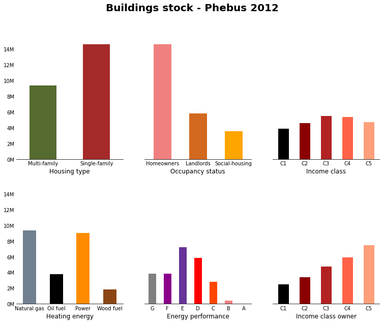
Fig. 1 Building stock 2012

Energy performance

The number of dwellings in each EPC band is directly given by Phébus-DPE.

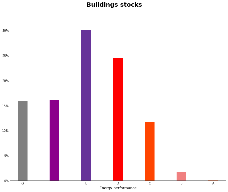
_images/buildingstock_ep_2012_percent.png

Fig. 2 Building stock 2012 by Energy Performance

Building characteristics and occupancy status

Table 3 specifies the joint distribution of building characteristics (singe- and multi-family dwellings) and types of investors (owner-occupied, landlord, social housing manager).

Table 3 Joint distribution of building and investor characteristics in Res-IRF 3.0
	Single-family	Multi-family	Total
Owner-occupier	49.00%	11.90%	60.90%
Landlord	8.80%	15.60%	24.40%
Social housing manager	3.20%	11.50%	14.70%
Total	61.00%	39.00%	100.00%

Heating fuel

The model covers energy use for heating from electricity, natural gas, fuel oil and fuel wood. This scope covers 16% of final energy consumption in France. We consider only the main heating fuel used in each dwelling. To identify it from the Phébus-Clode database, we proceed as follows:

We retain the main heating fuel when declared as such by the respondents.
When several main fuels are declared, we assign to the dwelling a heating fuel according to the following order of priority: district heating > collective boiler > individual boiler > all-electric > heat pump > other.
When no main fuel is reported, we retain the main fuel declared as auxiliary, determined with the following order of priority: electric heater > all-electric > mixed base > fixed non-electric > chimney.

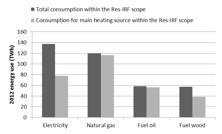
Fig. 3 Energy consumption in Phébus

Fig. 3 compares the total consumption of each fuel in the Phébus database and in the model. It shows that retaining only one fuel for each dwelling leads us to consider much less electricity and wood consumption than reported in Phébus. This is due for the most part to our exclusion of auxiliary heating, which predominantly uses electricity and wood, and to a lesser extent to our exclusion of the specific electricity consumption that is reported in Phébus.

Household income

A major advance of version 3.0, the introduction of income categories was intended to capture heterogeneity in:

the propensity of owners to invest in energy retrofits,
the intensity of use of heating infrastructure by occupants. The level of detail of the Phébus database made this development possible. Yet since the income data it contains only relates to occupants, additional data were needed to set income parameters for landlords.

Occupants

The disposable income of occupants – owner-occupiers and tenants – is segmented into five categories delineated by the same income boundaries as those defining income quintiles in France, according to the national statistical office for 2012. The use of these quintiles instead of those intrinsic in the Phébus sample ensures consistency between homeowners’ and tenants’ income (see next section), without introducing too strong biases, as shown in Table 4. Each dwelling is then allocated the average income for its category. Fig. 4 illustrates the distribution of occupant income in the different EPC bands. A clear correlation appears between household income and the energy efficiency of their dwelling.1

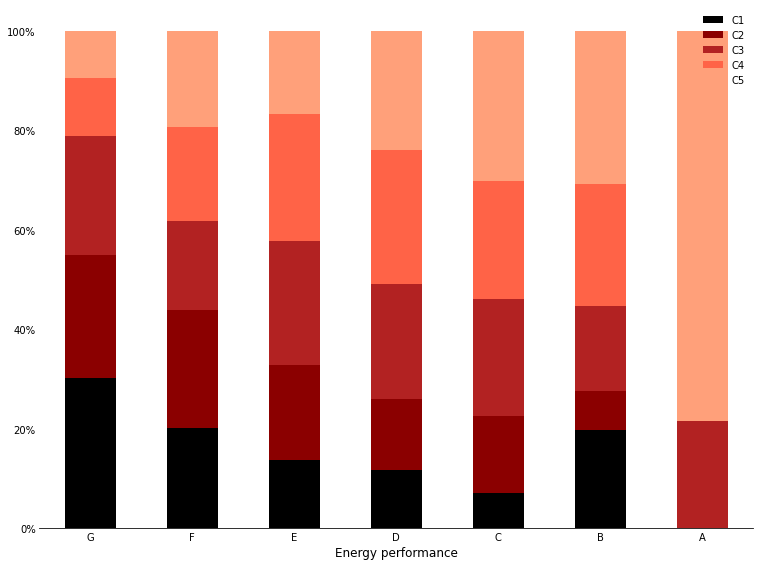
Fig. 4 Distribution of income categories within EPC bands. Source: Phébus

Table 4 Income categories used in Res-IRF 3.0
Category	Boundaries of Insee quintiles (€)	Share of total households in Res-IRF
C1	0 – 16,830	17%
C2	16,831 – 24,470	19%
C3	24,471 – 34,210	23%
C4	34,211 – 48,680	22%
C5	> 48,681	19%

Owners

Homeowners income overlaps with occupants. Yet Phébus does not contain any information on the income of landlords, which we had to reconstitute by other means. We matched the Phébus-DPE data with INSEE data pre-processed by the Agence nationale pour l’information sur le logement [ANIL, 2012]. The resulting landlords income distribution is described in Fig. 5 and compared to that of tenants. Here again, significant disparities appear, with households whose annual income falls below €34,210 representing 80% of tenants but only 20% of owner-occupiers.

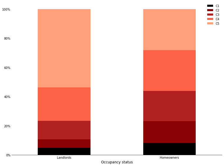
Fig. 5 Distribution of tenants income categories by occupancy-status.

To build this figure, some adjustments are needed to translate into income categories the [ANIL, 2012] data that are expressed in terms of living standard2.

Complete list of inputs

We use the term input to name any factor that is given a numerical value in the model. Model inputs fall into three categories [Branger, Giraudet, Guivarch, and Quirion, 2015]:

Exogenous input trajectories (EI) representing future states of the world: energy prices, population growth and GDP growth.
Calibration targets (CT), which are empirical values the model aims to replicate for the reference year. They include hard-to-measure aggregates such as the reference retrofitting rate and the reference energy label transitions.
All other model parameters (MP), which reflect current knowledge on behavioral factors (discount rates, information spillover rates, etc.) and technological factors (investment costs, learning rates, etc.)

Table 5 Complete list of inputs
Category	Input Name	Value 3.0	Source
Existing Dwelling Stock Factors	Initial building stock		Phebus, 2012
	Initial floor area (m2/dwelling)		Phebus, 2012
	Conventional consumption (kWh/m2/yr)		Phebus, 2012
Exogenous inputs	Energy Price (€/kWh)		ADEME, DGEC, EU
	Tax Price (€/kWh)	0
	Population Growth (%/yr)	0.30%	INSEE, 2006
	Growth in household income (%/yr)	1.20%	INSEE
Calibration targets	Retrofitting Rate (%)		PUCA, 2015
	Energy Label Transition Shares (%)		PUCA, 2015
	Construction Shares (%)		OPEN, 2016 ; USH, 2017
	Reference Energy Use (TWh)		CEREN, 2012
Innovation dynamics factors	Initial Capital Stock
	Learning Rate (%)	10%	Expert opinion
	Information Rate (%)	25%	Expert opinion
	Share of variable intangible costs (%)	95%	Expert opinion
	Share of variable intangible costs Construction (%)	80%	Expert opinion
Dwelling Stock Variation Factors	Household Density Growth	-0.007	Expert opinion
	Minimum Household Density (households/dwelling)	2	Expert opinion
	Floor area Elasticity		Expert opinion
	Maximum Floor area construction (m2/dwelling)		Expert opinion
	Initial Floor area construction (m2/dwelling)		Expert opinion
	Destruction Rate (%/yr)	0.35%	Expert opinion
	Proportion of Non-refurbishable Dwellings (%/initial stock)	5%	Expert opinion
	Mutation rate	%	Expert opinion
	Rotation rate	%	Expert opinion
Investment cost factors	Retrofitting Costs (€/m2)		Expert opinion
	Fuel Switch Costs (€/m2)		Expert opinion
	Construction Costs (€/m2)		Expert opinion
Other factors	Discount Rates (%/yr)		Expert opinion
	Discount Rate construction (%/yr)		Expert opinion
	Envelope Lifetime (yrs)		Expert opinion
	Heating System Lifetime (yrs)		Expert opinion
	New Dwellings Lifetime (yrs)	25	Expert opinion
	Heterogeneity Parameter	8	Expert opinion

Exogenous input

Energy prices: based on a scenario from ADEME using assumptions from the Directorate General for Energy and Climate ( DGEC) and the European Commission. The scenario used is equivalent to an average annual growth rate of fuel prices after tax of 1.42% for natural gas, 2.22% for fuel oil, 1.10% for electricity and 1.20% for fuel wood over the period. These lead to an average annual growth rate of the price index of 1.47%/year.
Population growth3: based on a projection from [INSEE, 2006] equivalent to an average annual growth rate of 0.3%/year over the period 2012-2050.
Growth in household income: extrapolates the average trend of 1.2%/year given by INSEE uniformly across all income categories.

Calibration target

Construction

Market shares used to calibrate intangible costs for construction.

Table 6 Market shares of construction in 2012.
Energy performance		BBC	BBC	BBC	BBC	BEPOS	BEPOS	BEPOS	BEPOS
Heating energy		Natural gas	Oil fuel	Power	Wood fuel	Natural gas	Oil fuel	Power	Wood fuel
Occupancy status	Housing type
Homeowners	Multi-family	71.5%	0.1%	17.6%	0.9%	7.9%	0.0%	2.0%	0.1%
Homeowners	Single-family	16.6%	0.5%	67.8%	5.2%	1.8%	0.1%	7.5%	0.6%
Landlords	Multi-family	71.5%	0.1%	17.6%	0.9%	7.9%	0.0%	2.0%	0.1%
Landlords	Single-family	16.6%	0.5%	67.8%	5.2%	1.8%	0.1%	7.5%	0.6%
Social-housing	Multi-family	71.5%	0.1%	17.5%	0.9%	7.9%	0.0%	1.9%	0.1%
Social-housing	Single-family	16.6%	0.5%	67.8%	5.2%	1.8%	0.1%	7.5%	0.6%

Intensive margin

Intangible costs are calibrated so that the life-cycle cost model, fed with the investment costs, matches the market shares reported here Table 7

Table 7 Market shares of energy efficiency upgrades in 2012. Source: PUCA (2015)
	F	E	D	C	B	A
G	25.00%	27.00%	27.00%	21.00%	0.00%	0.00%
F		40.40%	26.30%	31.30%	2.00%	0.00%
E			66.00%	28.00%	6.00%	0.00%
D				95.00%	5.00%	0.00%
C					90.90%	9.10%
B						100.00%

In the absence of any substantial improvement in the quality of the data available, the matrix remains unchanged from version 2.0 of the model.

Extensive margin

Parameter ρ (of renovation function) is calibrated, for each type of decision-maker and each initial label (i.e., 6x6=36 values), so that the NPVs calculated with the subsidies in effect in 2012 [Giraudet, Guivarch, and Quirion, 2012] reproduce the renovation rates described in Table 8and Table 9 and their aggregation represents 3% (686,757 units) of the housing stock of the initial year.

Table 9 Renovation rate by type of dwelling. Source : OPEN (2016) and USH (2017)
Type of decision-maker	Type of dwelling	Renovation rate
Owner-occupied	Single-family	4.70%
	Multi-family	3.60%
Privately rented	Single-family	2.00%
	Multi-family	1.80%
Social housing	Single-family	1.50%
	Multi-family	2.00%

Aggregated energy consumption

To ensure consistency with the CEREN data, which is the reference commonly used in modelling exercises, Res-IRF is calibrated to reproduce the final energy consumption given by CEREN for each fuel in the initial year. The resulting conversion coefficients applied to the Phebus Building Stock are listed in Table 10.

Table 10 Calibration of total final actual energy consumption
	Electricity	Natural gas	Fuel oil	Fuel wood	TOTAL
CEREN values to be reproduced in 2012 (TWhEF)	44.4	119.7	55.5	73.3	292.9
Correction factor applied to Res-IRF 3.0	0.79	1.06	1.03	2.14	1.14

Dwelling Stock Variation Factors

Table 11 Initial Floor area construction (m2/dwelling)
	Single-family	Multi-family
Homeowners	132	81
Landlords	90	60
Social-housing	84	71

Table 12 Floor area construction elasticity
	Single-family	Multi-family
Homeowners	0.2	0.1
Landlords	0.2	0.1
Social-housing	0.1	0.1

Table 13 Maximum Floor area construction (m2/dwelling)
	Single-family	Multi-family
Homeowners	160	89
Landlords	101	76
Social-housing	90	76

Table 14 Rotation and Mutation rate (%/year)
	Rotation rate	Mutation rate
Homeowners	18.0%	1.8%
Landlords	3.5%	0.0%
Social-housing	8.0%	0.3%

Investment cost factors

Table 15 Renovation costs used in Res-IRF 3.0 (€/m2). Source: Expert opinion
	F	E	D	C	B	A
G	76.0	136.2	200.6	270.7	350.5	441.9
F		63.0	130.3	203.5	286.7	381.8
E			70.0	146.0	232.3	330.9
D				79.0	168.6	270.7
C					93.0	198.9
B						110.0

The matrix equally applies to single- and multi-family dwellings, in both private and social housing. In the absence of any substantial improvement in the quality of the data available, the matrix remains unchanged from version 2.0 of the model.

Table 16 Switching-fuel costs used in Res-IRF 3.0 (€/m2). Source: Expert opinion
Heating energy	Power	Natural gas	Oil fuel	Wood fuel
Power	0	70	100	120
Natural gas	55	0	80	100
Oil fuel	55	50	0	100
Wood fuel	55	50	80	0

Table 17 Construction costs (€/m2)
Heating energy final	Power	Power	Natural gas	Natural gas	Oil fuel	Oil fuel	Wood fuel	Wood fuel
Energy performance final	BBC	BEPOS	BBC	BEPOS	BBC	BEPOS	BBC	BEPOS
Single-family	979	1112	1032	1059	1032	1059	1094	1121
Multi-family	1199	1308	1242	1253	1242	1253	1323	1350

Existing Dwelling Stock Factors

Table 18 Initial Floor area (m2/dwelling)
	Single-family	Multi-family
Homeowners	123	76
Landlords	90	52
Social-housing	84	66

Table 19 Income (€/year)
	Income class
C1	14103
C2	21002
C3	29394
C4	41091
C5	61300

Other factors

Table 20 Discount rates (%/year). Source: Expert opinion
Income category	Single-family housing	Multi-family housing	Social housing
C1	15%	37%	4%
C2	10%	25%	4%
C3	7%	15%	4%
C4	5%	7%	4%
C5	4%	5%	4%

Table 21 Investment horizon (years). Source: Expert opinion
Scenario	Homeowners	Landlords	Social-housing
Full capitalization	30 (16) years	30 (16) years	30 (16) years
Reference	30 (16) years	3 years	30 (16) years
No capitalization at resale	7 years	7 years	30 (16) years
No capitalization in rents nor sales	7 years	3 years	30 (16) years

Considering that the quality of new constructions results from decisions made by building and real estate professionals rather than by future owners, we subject these decisions in the model to private investment criteria, reflected by a discount rate of 7% and a time horizon of 35 years.

Table 22 Discount rates construction (%/year). Source: Expert opinion
Occupancy status	Single-family housing	Multi-family housing
Homeowners	7%	10%
Landlords	7%	10%
Social housing	4%	4%

Appendix

Fig. 6 Building stock 2012 (%)

1: The low number of dwellings labelled A and B in Phébus makes income distribution statistics less accurate in these bands.
2: This metric divides household income by consumption units – 1 for the first adult, 0.5 for any other person older than 14 and 0.3 for any person under that age. It is generally thought to better represent the financing capacity of a household than does income.
3: The population is adjusted by a factor of 23.9/27.1 to take into account the difference in scope between Res-IRF and Phébus. The resulting average household size is 2.2 persons per dwelling in 2013, a value consistent with [INSEE, 2017]; it decreases with income to reach 2.05 in 2050.