Simulation and sensitivity analysis

Influence of exogenous variables

The influence of technological progress, energy prices and aggregate household income is assessed by comparing the reference scenario to alternatives in which they are frozen one after the other1.

Table 36 Scenario specification
Scenario	Endogenous techological change	Energy prices	Housholds income
Reference	Learning rate of 15% for new construction and 10% for renovation.	ADEME scenario	Growth rate of 1,2%/yr
No technological change	Frozen. Learning rates set to zero.	ADEME scenario	Growth rate of 1,2%/yr
No technological change, frozen price	Frozen. Learning rates set to zero.	Frozen	Growth rate of 1,2%/yr
No technological change, frozen price and income	Frozen. Learning rates set to zero.	Frozen	Frozen

Fig. 10 illustrates the resulting effect on the aggregate final energy consumption for heating, the main output of the model. It shows that energy consumption decreases autonomously from 15% to 30%, depending on the scenarios considered, between 2012 and 2050. Freezing technological progress increases energy consumption by 12% in 2050 relative to the reference scenario. Additionally, freezing energy prices further increases energy consumption by 20%. Lastly, freezing income decreases energy consumption by another 15%.

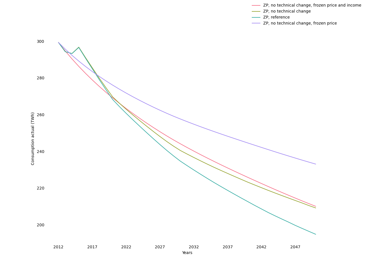
Fig. 10 Evolution of final actual energy consumption

Fig. 11 and Fig. 12 illustrate effects on the intensive and extensive margin of renovation. Fig. 11 shows that freezing technological progress significantly reduces the annual flow of renovations. Additionally freezing energy prices reinforces this effect, while freezing income has no additional effect. The declining trend observed in the all-frozen scenario illustrates the depletion of the potential for profitable renovations as a result of past renovations. The comparison with the other scenarios shows that technological progress and, to a lesser extent, increasing energy prices are augmenting this potential. Fig. 12 shows that the scenarios with the highest number of renovations generate fewer numbers in the low-efficiency labels (G to C) and more in high-efficiency ones (B and A).

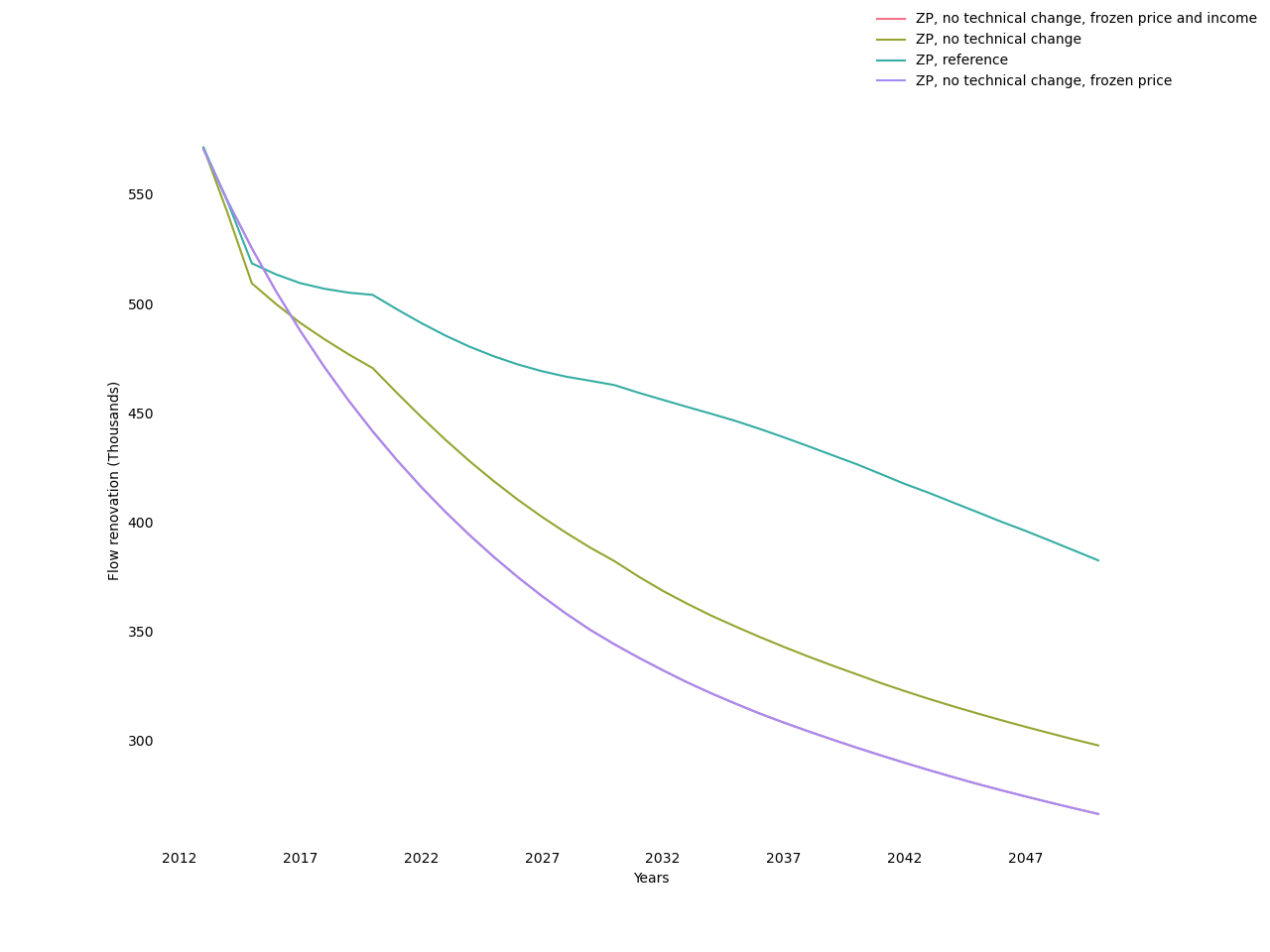
Fig. 11 Renovation flows

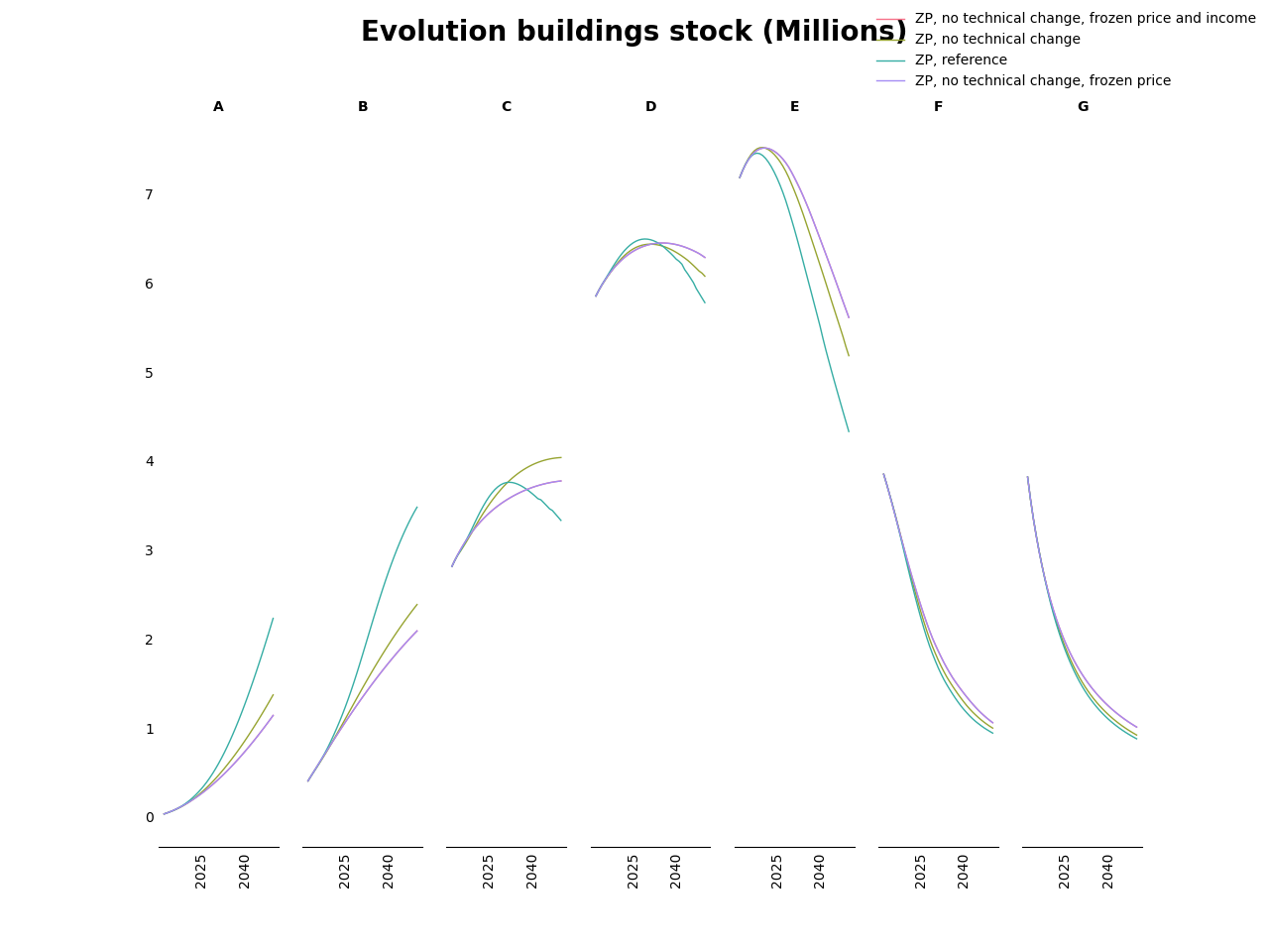
Fig. 12 Evolution of energy performance

The aggregate heating intensity decreases with the theoretical budget share dedicated to heating Fig. 13, which in turn decreases with the energy performance of the dwelling, decreases with household income and increases with the price of energy. The effect of the energy price on this quantity is ambiguous since, in addition to the direct effect just mentioned, there is the indirect effect discussed in the previous paragraph that the energy price stimulates renovations. The fact that the curve with non-frozen energy prices crosses that with frozen energy prices (both with frozen technological change) suggests that the direct effect dominates in the short term while the indirect effect dominates in the long term. The comparison of the first two scenarios indicates that freezing technological change reduces heating intensity, an effect due, as we have seen previously, to a lesser improvement in energy efficiency. Finally, the comparison of the last two scenarios illustrates the positive effect of income growth on heating intensity. It is important to note that, at the same time, the growth in aggregate income increases the surface area of dwellings to be heated.

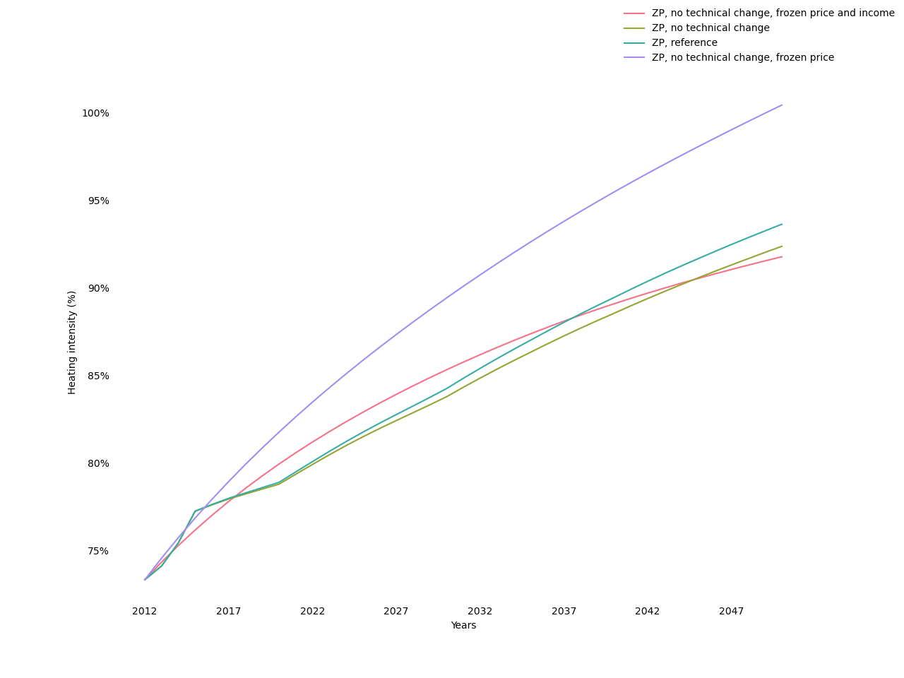
Fig. 13 Evolution of heating intensity

To sum up:

The reduction in energy consumption is to a large extent autonomous, that is, important even when all key drivers are frozen;
The rise in energy prices stimulates renovation and reduces intensity of heating; the former effect tends to take over the latter in the long term;
Technological progress has a pure effect of improving energy efficiency;
Income growth increases energy consumption by increasing both the area to be heated and the intensity of heating.

Fig. 14 displays the evolution of the share of dwellings in fuel poverty, as measured by the income-to-price ratio that counts the households spending more than 10% of their income on heating. It shows that, when all key drivers are frozen, this count consistently declines. The increase in income naturally accelerates this trend, while the increase in energy prices does the opposite. In comparison, technological change has a modest effect on reducing fuel poverty.

Fig. 14 Number of households dedicating over 10% of their income to heating

Influence of the determinants of capitalization

Table 37 Scenario specification capitalization
Scenario	Homeowners	Landlords	Social-housing
Full capitalization	30 (16) years	30 (16) years	30 (16) years
Reference	30 (16) years	3 years	30 (16) years
No capitalization at resale	7 years	7 years	30 (16) years
No capitalization in rents nor sales	7 years	3 years	30 (16) years

Here we compare the four scenarios specified in Table 37 (the scenario without the landlord-tenant dilemma corresponding to full capitalization). The absence of capitalization results in a reduction in the number and quality of renovations Fig. 15 and Fig. 16; even if this trend induces a counter-rebound effect Fig. 17, it results in an increase in aggregate energy consumption Fig. 18. The absence of capitalization in rents has a similar effect, although much weaker. In contrast, under the assumption of full capitalization, whereby landlords have the same willingness to invest as owner-occupiers, energy efficiency improvements and, ultimately, energy savings are more important than in reference.

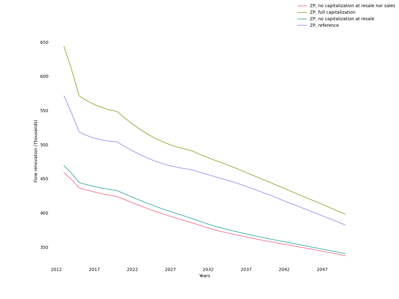
Fig. 15 Renovation flows

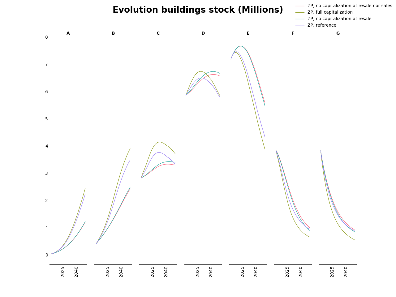
Fig. 16 Evolution of energy performance

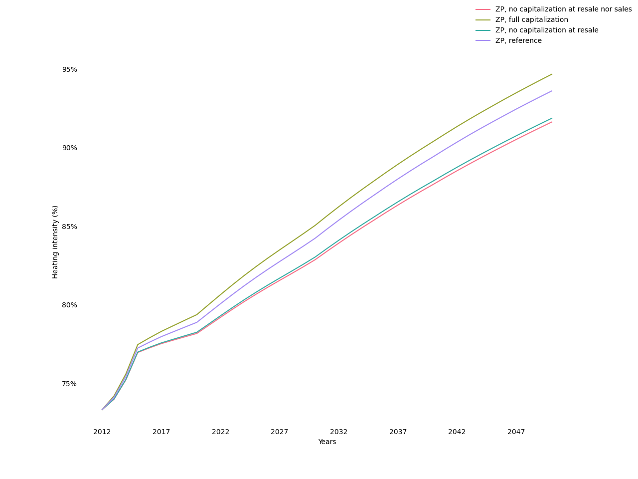
Fig. 17 Evolution of heating intensity

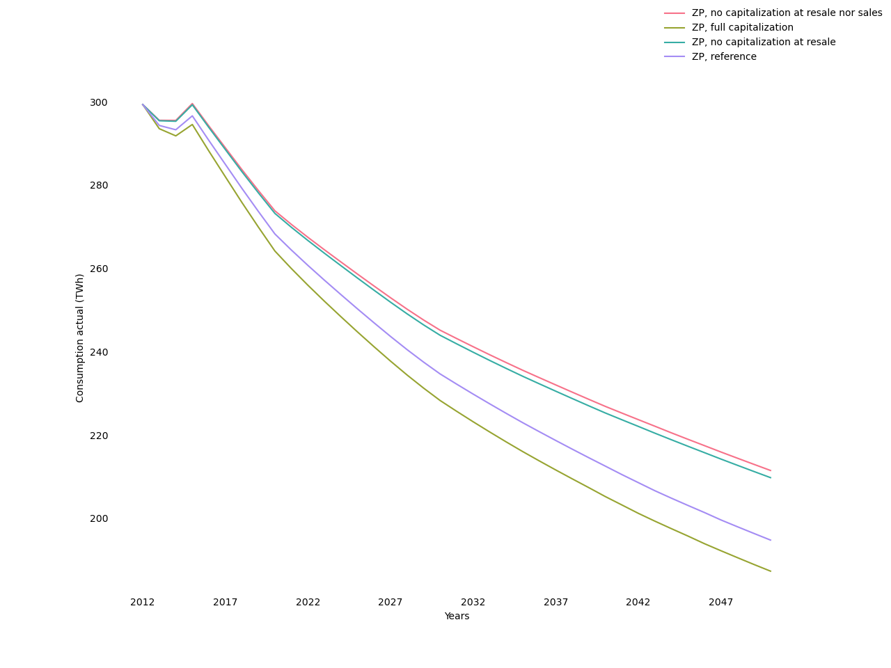
Fig. 18 Evolution of final actual energy consumption

Influence of credit constraints

To assess the influence of credit constraints, we set discount rates as follows:

Reference: the discount rates are those described in Table 34;
No credit constraints: all discount rates are equal to 7%;
Public investment: all discount rates are equal to 4%.

As shown in the following figures, these variants have relatively modest effects on renovation dynamics and aggregate consumption. Credit constraints therefore do not seem to play a major role in the model. This result is consistent with the conclusions of the sensitivity analysis to which Res-IRF 2.0 was subjected [Branger, Giraudet, Guivarch, and Quirion, 2015].

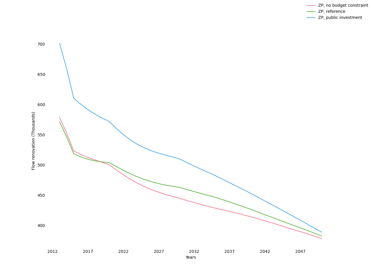
Fig. 19 Renovation flows

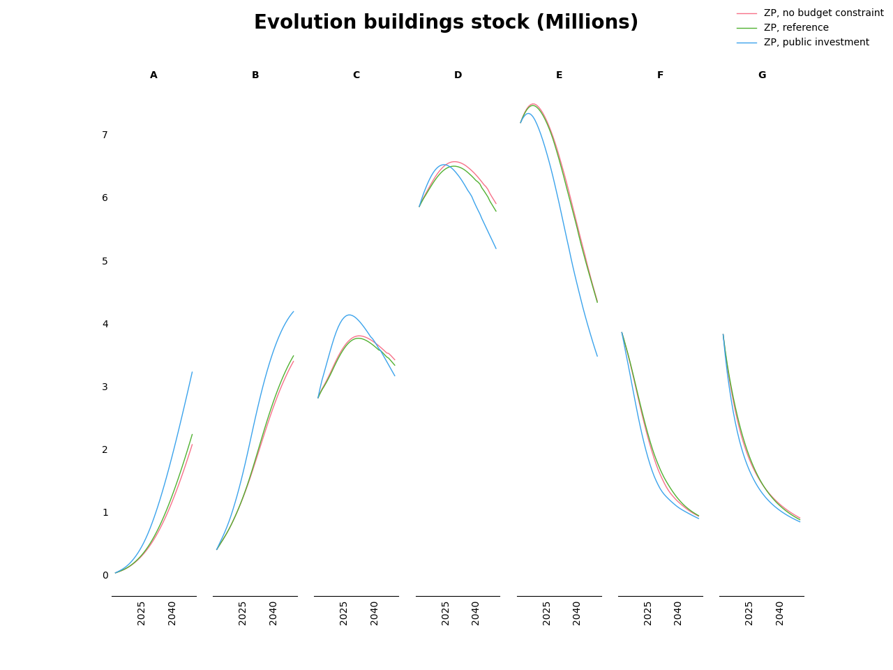
Fig. 20 Evolution of energy performance

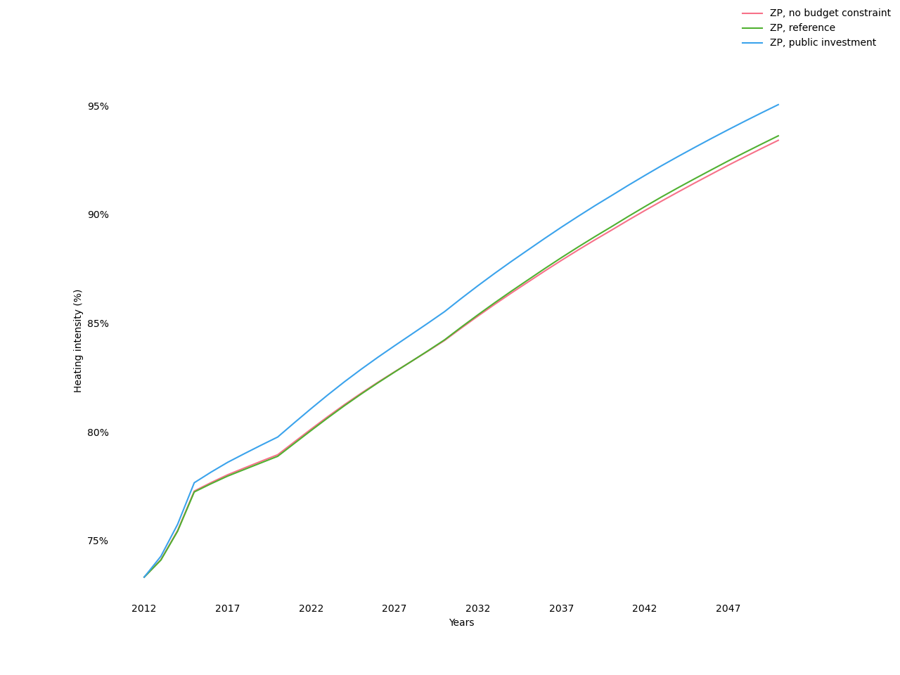
Fig. 21 Evolution of heating intensity

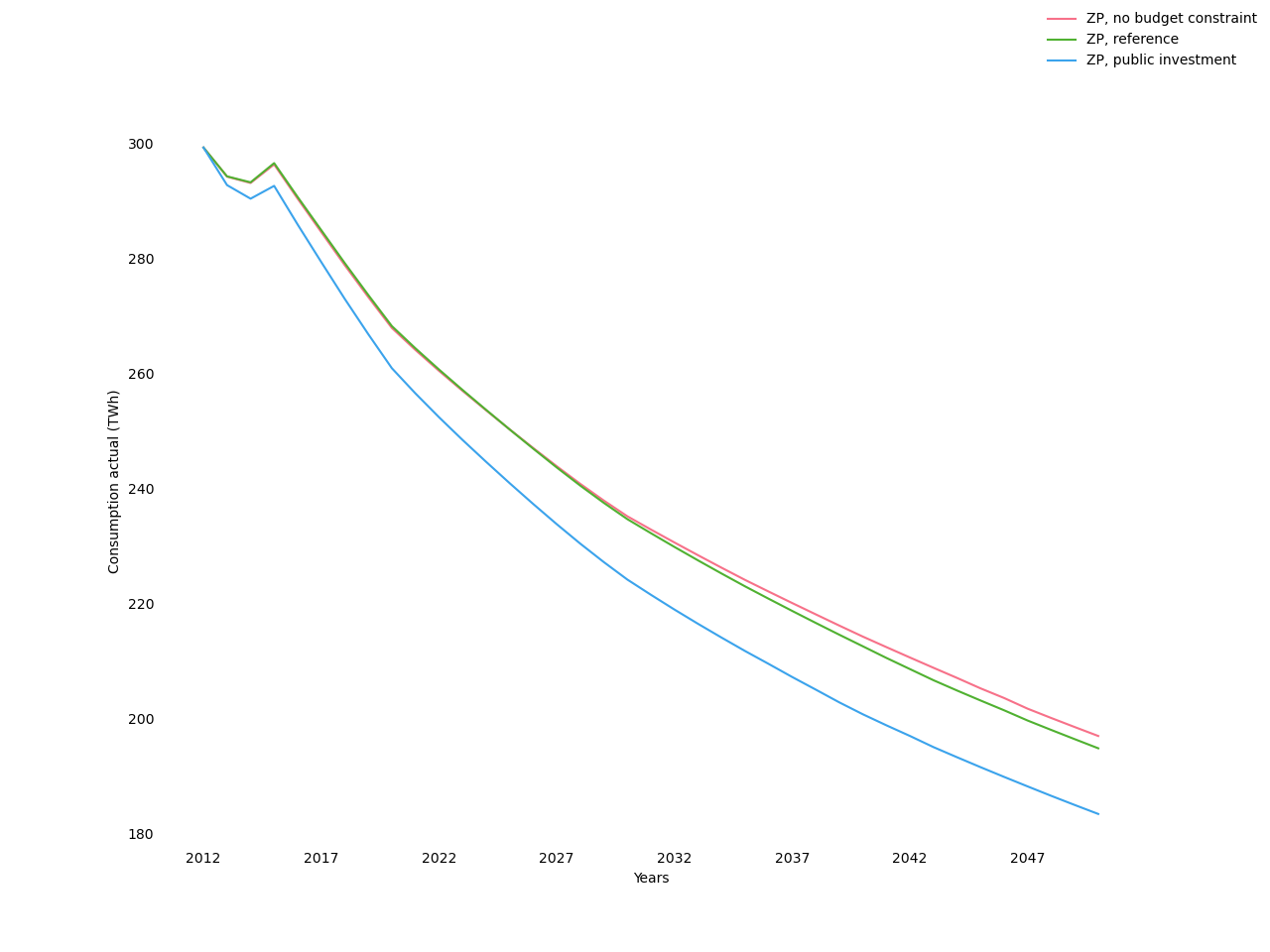
Fig. 22 Evolution of final actual energy consumption

1: Changing the order in which the variables are frozen has little impact, which suggests that non-linearities are not too important in the model.